Measuring noise figure using Gain Method

For those into radio astronomy would know the significance of having ultra-low noise figures. Lower the noise figure, the more sensitive your receiver becomes. Noise figure is a unit of measure that tells us how much noise, for example, your amplifier is adding to the signal at its input. All devices add some amount of noise to the signal passing through them. Our intention is always to keep this noise figure low. All that is fine, but how do you measure this noise figure? Well, there are several techniques that require special equipment. For example, a calibrated noise source while using the noise source method. On the other hand, liquid nitrogen while using the Y-Factor method. Keeping all that aside, I found that measuring noise figure using the Gain method to be the simplest.

The noise floor

There’s a very basic law that states that wider the bandwidth the noisier it gets. Fellow ham radio operators would easily correlate this. Remember that when you switch your HF radio set to CW mode, the noise suddenly reduces. On the other hand, if you switch to AM, the noise level rises. I have a Yaesu FT-450D which allows me to change the bandwidth of the receiver. The moment I reduce the bandwidth, it gets a little less noisy. I reduce some more and the noise reduces further. I have been quite subjective so far in terms of noise. So, speaking more on absolute terms, you should be looking at the S-meter on your radio set.

On a small filter bandwidth, the S-meter shows a certain noise level, say S2. Increase your bandwidth and it becomes S4. Increase it further and it might become S6. To explain it mathematically, the noise power and the bandwidth relation is expressed as below:

\(N_p = kTB /Hz\)

\(k = Boltzmann \,Constant = 1.38 \times 10^{-23}\)

\(T = Temperature\, in\, degrees\, K = 298.5^o K\)

\(B = Bandwidth = e.g. 1 Hz\)

Note that, the result will be a very very small number. To make things a bit humanly readable, we apply log.

\(N_p(dBm) = 10log(kTB)/Hz\)

Using this equation, we can find the noise power for various bandwidths.

\(\begin{array} {|r|r|}\hline 1Hz & -174\, dBm/Hz \\ \hline 10Hz & -164\, dBm/Hz \\ \hline 100Hz & -154\, dBm/Hz \\ \hline 1kHz & -144\, dBm/Hz \\ \hline 10kHz & -134\, dBm/Hz \\ \hline 100kHz & -124\, dBm/Hz \\ \hline 1MHz & -114\, dBm/Hz \\ \hline 10MHz & -104\, dBm/Hz \\ \hline \end{array}\)

To type the entire thing on a calculator is tedious, there is a simpler expression which takes \(-174\,dBm/Hz\) as the base and adds on top of it.

\(-174 + 10log(B) \,dBm/Hz \,…where\, B\, is\, bandwidth\, in\, Hz\)…(*)

Doing the measurement

Now that we have tried to understand the relation between noise and bandwidth, let us try to use that for measuring the noise figure. In this experiment, I will be using an old Agilent E4400B spectrum analyzer. The DUT (Device under test) will be cascaded Minicircuits PSA4-5043+ low noise amplifier. We will be using a very simple equation to calculate the noise figure which is as follows:

\(NF = N_{P_{device}} – (-174+10log(B)+Gain)\)

…where \( N_{P_{device}}\) is the noise power when the device is powered up. Read further to find out how we can measure this.

The settings:

• Resolution bandwidth: 1kHz. This is the minimum I can go on this instrument.
• Video bandwidth: 1kHz. Changing this will change the displayed noise level in spite of having a low RBW.
• Centre frequency: 1GHz
• Span: 100kHz

The process

• Find \( N_{P_{device}}\) (Device is powered on)
• Find Gain
• Calculate NF using the above equation (*)

First, we need to measure the noise level coming out of the device when it’s turned on. This parameter is \( N_{P_{device}}\) as denoted earlier. First, adjust the spectrum analyzer to the settings given above. Then connect the DUT to the spectrum analyzer input and power it on. Make sure the DUT input is terminated in \(50\Omega\).

Observe the noise floor level and note it down.

Noise floor when the device under test is powered on. Ignore the peak on the side. No idea where that pickup is coming from.

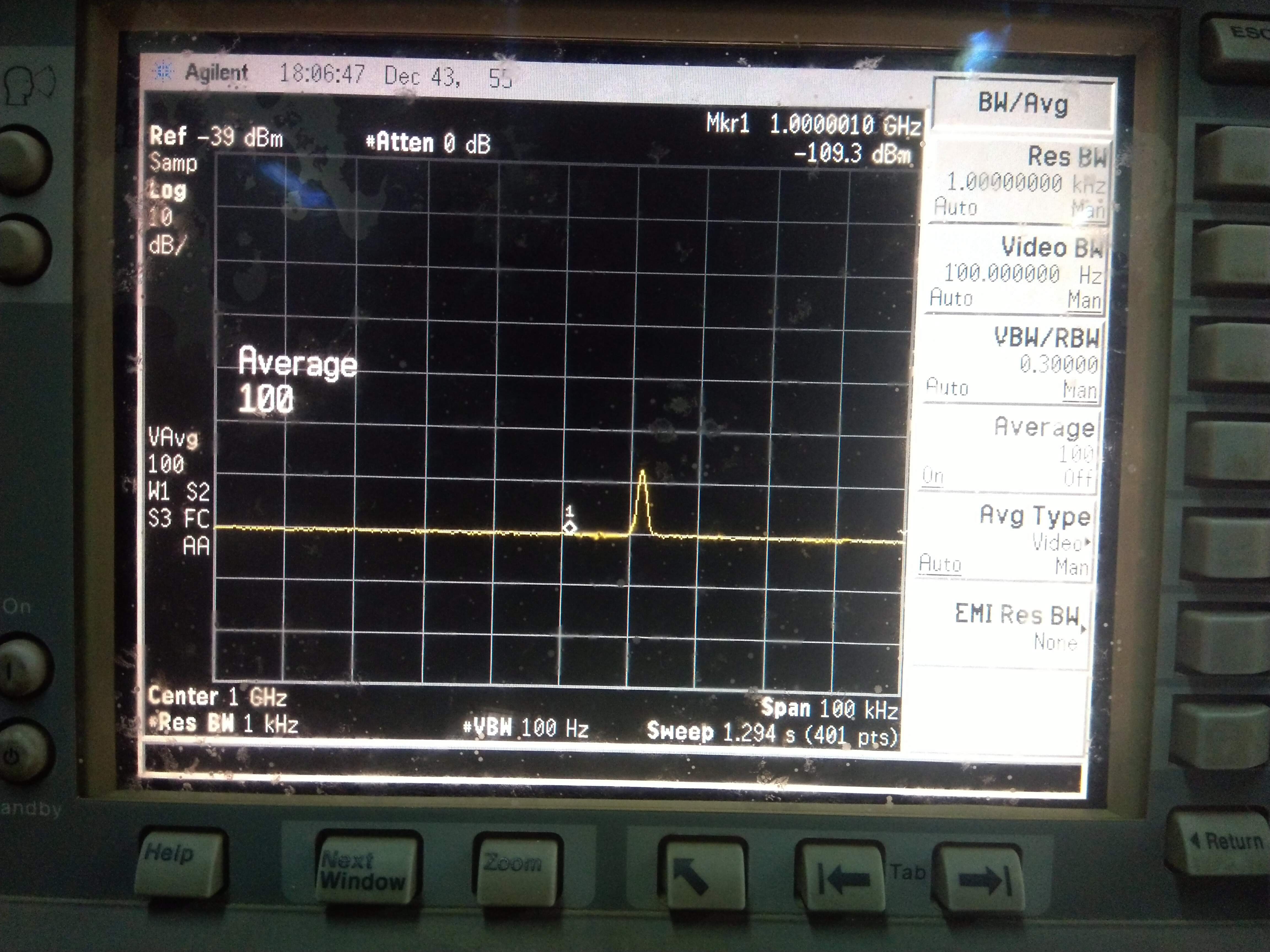
Based on the observation, the noise floor power level is \(-109.3 \,dBm\).

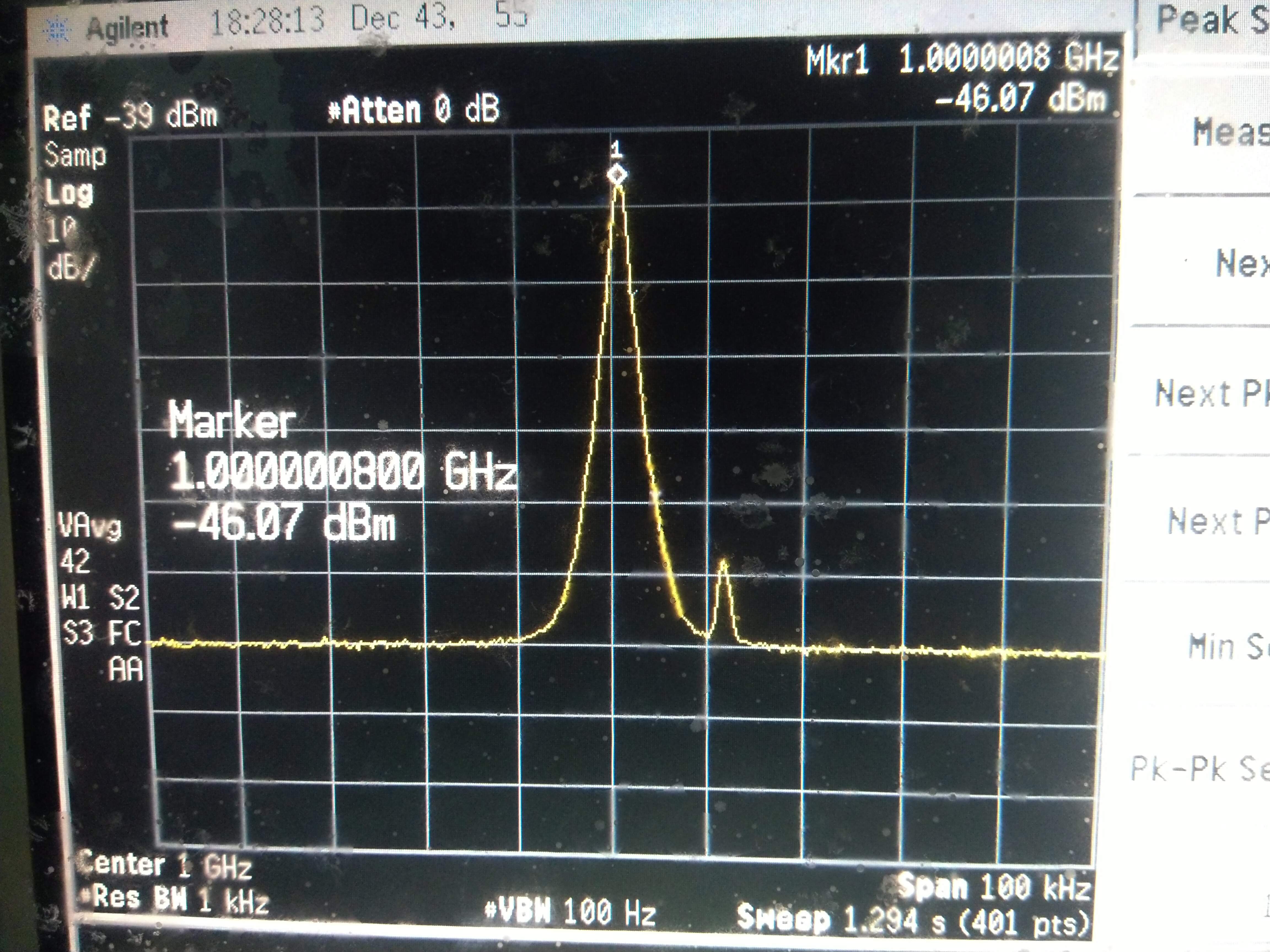
Now, apply 1GHz RF signal at the input and power output. Based on that, we will calculate the gain of the device. In my case, I applied a 1GHz signal with \(-80\,dBm\) power.

Output of the DUT when 1GHz signal of -80dBm power provided at the input of DUT

As one can see, the DUT pumps out \(-46\,dBm\) power. Based on this, we can calculate the gain of our DUT.

\(Gain = P_{out}-P_{in} = -46.07 – (-80) = 33.93\,dB\)

Using the equation given somewhere above, we must calculate the noise figure.

\(NF = -109.3-(-174+10log(1kHz)+33.93) = 0.77\,dB\)

Conclusion

Before we conclude, let us compare the data given in the datasheet.

Data from the official datasheet

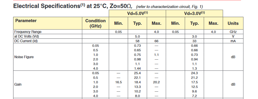
Based on the information in the datasheet, we can see that the noise figure at 1GHz is typically 0.75 dB. Our calculation also results in a value very close to the given data.

Measured NF: 0.77 dB

Given NF: 0.75 dB

The only drawback of this method is that you require a DUT having a gain that can cause measurable change in the displayed noise floor.

In a future article, we will try to understand how noise figure is an important factor that affects every radio operator.