
Radar Beamforming to track target
he Matlab phased array toolbox is a collection of many interesting algorithms and functions. With so many tools at your disposal, the phased array toolbox lets us build a complete end to end radar system. I tried the phased array toolbox for the first time to build a pulsed radar which can determine approximate azimuth angle of the target with respect to the radar.
Setting up the stage
In order to simulate a radar system in Matlab, you need to have everything defined. For example, the transmitter, the antenna system, the target itself and so on. Let us define a few things related to the radar before we proceed.
System specifications
Our operating frequency will be 9850MHz. The transmit power will be set at 5W and receiver preamplifier gain set to 10dB with a noise figure of 5. Additionally, we shall be transmitting a pulse with Linear frequency modulation for pulse compression. The LFM pulse will have sweep bandwidth of 5MHz. The radar pulse repetition frequency would be set to 10kHz resulting in a maximum unambiguous range of 15km.
\(R_{max} = \frac{c}{2 \times PRF}\)
Our pulse width will be equal to \(1\mu s\) resulting in a range resolution of,
\(\Delta R = \frac{c\times pulse width}{2} = 150 meters\)
Since we are going to transmit an LFM pulse, our range resolution increases. Higher the sweep bandwidth, higher is the pulse compression ratio (PCR) and better the range resolution gets.
\(\Delta R = \frac{c}{2 \times B} = 30 meters\)
A staggering improvement in range resolution by a factor of 5. Further in this article we will also see how LFM improves the detection probability as compared to an unmodulated pulse.
The antennas
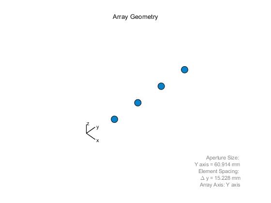
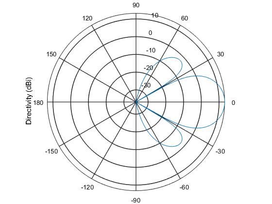
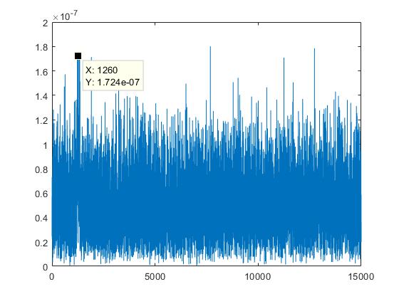
We begin by setting up a simple array antenna. In this example, we will use a Uniform Linear Array having 4 radiating elements. Below, we see the arrangement of the antenna array as well as its radiation pattern.
|
1 2 3 4 5 6 7 8 9 10 |
antenna=phased.ULA; antenna.NumElements = 4; cosineElement = phased.CosineAntennaElement; antenna.Element = cosineElement; antenna.ElementSpacing = (3e8/9850e6)/2; OpFreq = 9850e6; viewArray(antenna); pattern(antenna,OpFreq,-180:180,0,... 'Type','directivity',... 'PropagationSpeed',3e8) |
Next, we set up the transmit waveform as follows.
|
1 2 3 4 5 6 7 8 9 10 11 |
% Waveform Specs waveform=phased.LinearFMWaveform; waveform.SweepBandwidth = 5e6; waveform.SampleRate = 100e6; % 100 MHz sample rate waveform.PRF=10000; % Pulse Repetition Frequency of 10000 pulses per second waveform.PulseWidth=1e-6; % Pulse width of 1us nSamples = waveform.SampleRate/waveform.PRF; % Define pulses on 10000 samples b = getMatchedFilter(waveform); matchedFilter = phased.MatchedFilter('Coefficients', b, 'SpectrumWindow','Hamming') y = step(waveform); t = (0:nSamples-1)/waveform.SampleRate; |
Along with the waveform, we also initialize our matched filter coefficients in this code.
Next, we place a target parameters using the following code,
|
1 2 3 4 5 6 7 8 9 10 11 12 13 14 15 16 17 |
% Transmitter Specs for amplification TX=phased.Transmitter('Gain',20); TX.PeakPower = 50; % Target Specs TgtModel=phased.RadarTarget; TgtModel.MeanRCS = 0.1; TgtModel.OperatingFrequency = OpFreq; tgtDistance = 1.2e3; tgtAz = 0.25; tgtPos=[cos(tgtAz)*tgtDistance;sin(tgtAz)*tgtDistance;0]; % Target at 1.2 km distance, 14.3 degree azimuth tgtVel=[75*cos(tgtAz);75;0]; % Radial velocity is 150 m/sec % Platform Specs PlatformModel=phased.Platform; PlatformModel.InitialPosition = tgtPos; PlatformModel.Velocity = tgtVel; |
The target is set to have an RCS of 0.1 square meters located at an azimuth angle of 0.25 radians (~14.3 degrees) and 1.2 km away.
When we transmit our radar pulse, it propagates through the free space, hits the target and returns. The electromagnetic waves decay at a rate governed by square law. Also, the channel behaves differently for different frequencies. Therefore, we need to set the channel parameters as well to get a realistic result.
|
1 2 3 4 5 |
% Channel Specs ChannelModel = phased.FreeSpace; ChannelModel.TwoWayPropagation=true; ChannelModel.OperatingFrequency = OpFreq; ChannelModel.SampleRate = waveform.SampleRate |
Transmitting the pulses
Most of the things that we need are ready for action. We shall send 64 pulses and receive them to form a radar data cube.
|
1 2 3 4 5 6 7 8 9 10 11 12 13 |
for ii=1:nPulses wf=step(waveform); % Generate waveform [tgtPos, tgtVel] = step(PlatformModel,1/prf); % Update target position [~, tgtAng] = rangeangle(tgtPos, radarPos); % Calculate range/angle to target s0 = step(TX, wf); % Amplify signal s1 = step(txArray,s0, tgtAng); % Radiate the signal from the array s2 = step(ChannelModel, s1, radarPos, tgtPos, radarVel, tgtVel); % Propagate from radar to target and return s3 = step(TgtModel, s2); % Reflect signal from Target s4 = step(rxArray,s3,tgtAng); % Receive the signal at the array s5 = step(rxPreamp,s4); % Add rx noise datacube(:,:,ii) = s5(:,:); % Build data cube 1 pulse at a time end |
At the end of the loop, we end up with a 3-dimensional matrix containing data from 4 receive channels with a sample length of 10000 and we do this for 64 pulses.
Based on this data cube, we can steer the receiver channels to look in certain direction. For example, we can digitally focus on \(30^o\) azimuth and observe the data in that direction. Let us try that.
First, we initialize a beamformer object to steer the main lobe towards \(30^o\) azimuth. Apply the beamforming over one pulse width data samples and observe it’s output.
|
1 2 3 4 |
beamformer3 = phased.PhaseShiftBeamformer('SensorArray', antenna, ... 'OperatingFrequency',OpFreq, 'Direction', [30; 0]); bf3 = beamformer3(datacube(:, :, 13)); plot(t(1:10000), abs(bf3)); |
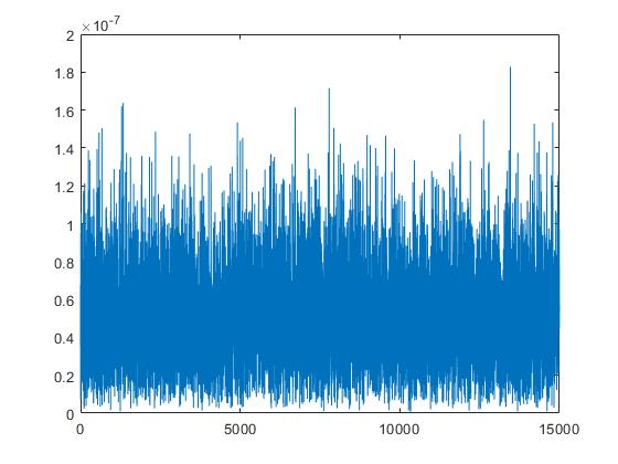
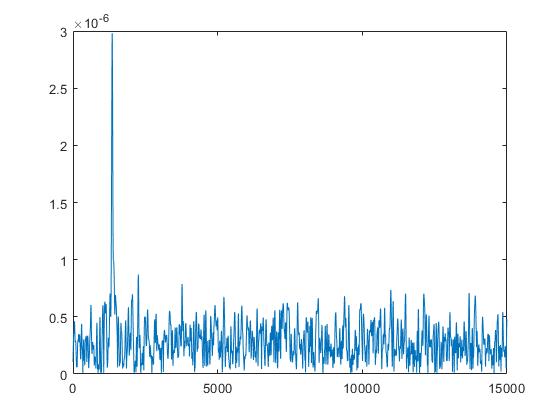
Clearly, the pulse is hardly visible in this noisy plot. Based on what I said earlier, the modulated pulse helps increase the probability of target detection. By running a matched filter over this data, we will see if we can extract anything out of this.
|
1 2 |
mf = abs(step(matchedFilter, bf3)); plot(t, mf); |
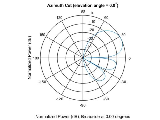
Now, let us steer the beam to 15 degrees (close to where our target is located) and observe the antenna pattern as well as the processed data output. Ideally, we should see that the detected pulse has a higher amplitude as compared to when we looked towards \(30^o\) azimuth.
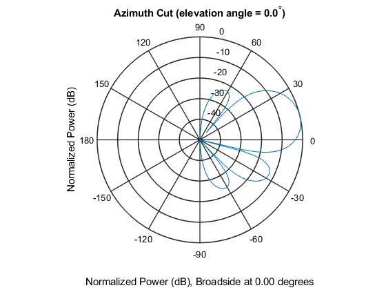
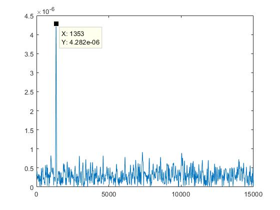
Comparing the raw data, we can see an increased amplitude of the reflected pulse when we beamform at \(15^o\) azimuth. Correspondingly, the matched filter output also shows a better peak amplitude.
Basic tracking
A very basic target tracking algorithm works by transmitting two pulses which are slightly offset in either azimuth or elevation (whichever direction you want to track, most of the times both directions). This technique is known as lobing. We can do a similar thing digitally over our radar data cube. The only thing required is that the target should fall in our main lobe.
First, I did a steered the beam towards \(20^o\) and then another beam \(4^o\) apart. We collect the data from both the beams, run a matched filter over it and observe the obtained target peaks as follows.
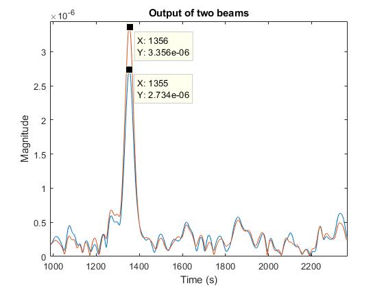
Had the targets been centred in the main lobe (boresight), we would see equal amplitudes. Over the next few iterations, we try to minimize the difference by increasing the beam azimuth angle.
Remember that we are not changing the axis of our radar platform anywhere but simply working on the radar data cube we obtained previously.
|
1 2 3 4 5 6 7 8 9 10 11 12 13 14 15 16 17 18 19 20 21 22 23 24 25 26 |
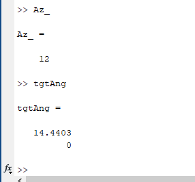
for ii=1:nPulses % First beam beamformer1 = phased.PhaseShiftBeamformer('SensorArray',antenna,... 'OperatingFrequency',OpFreq,'PropagationSpeed',3e8,... 'Direction',[Az_;0],'WeightsOutputPort',true); % Second offset beam beamformer2 = phased.PhaseShiftBeamformer('SensorArray',antenna,... 'OperatingFrequency',OpFreq,'PropagationSpeed',3e8,... 'Direction',[Az_ + 4;0],'WeightsOutputPort',true); [bf0(:, ii), w0] = beamformer1(datacube(:, :, ii)); [bf1(:, ii), w1] = beamformer2(datacube(:, :, ii)); % Match filter both beams matchFiltered1(:, ii) = abs(step(matchedFilter, bf0(:,ii))); matchFiltered2(:, ii) = abs(step(matchedFilter, bf1(:,ii))); [pk1, idx] = max(matchFiltered1(:,ii)); pk2 = max(matchFiltered2(:,ii)); if (pk1 - pk2) > 0 Az_ = Az_ - 0.5; end if (pk1 - pk2) < 0 Az_ = Az_ + 0.5; end end |
Eventually, the two target peaks become equal and finally end up with Az_ value close to the actual target position.
Conclusion
I am just now learning concepts of MIMO, phased array radars and target tracking. I toyed around the Matlab phased array toolbox to get my hands dirty. There is a Monopulse target tracking algorithm which is widely used and my next post could be about that. It allows us to accurately track moving targets.
Additionally, we can also steer the transmit beam and obtain much better results. That is when we would enter the realm of active electronic scan arrays.
For those who want the code, email me.
Really interesting….gr8 job Master Salil