
Cable impedance profile with NanoVNA and TDR script
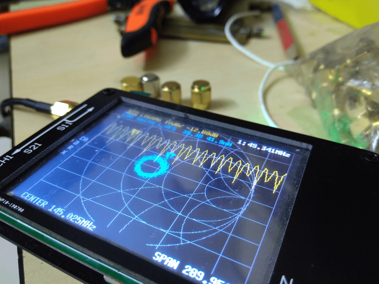
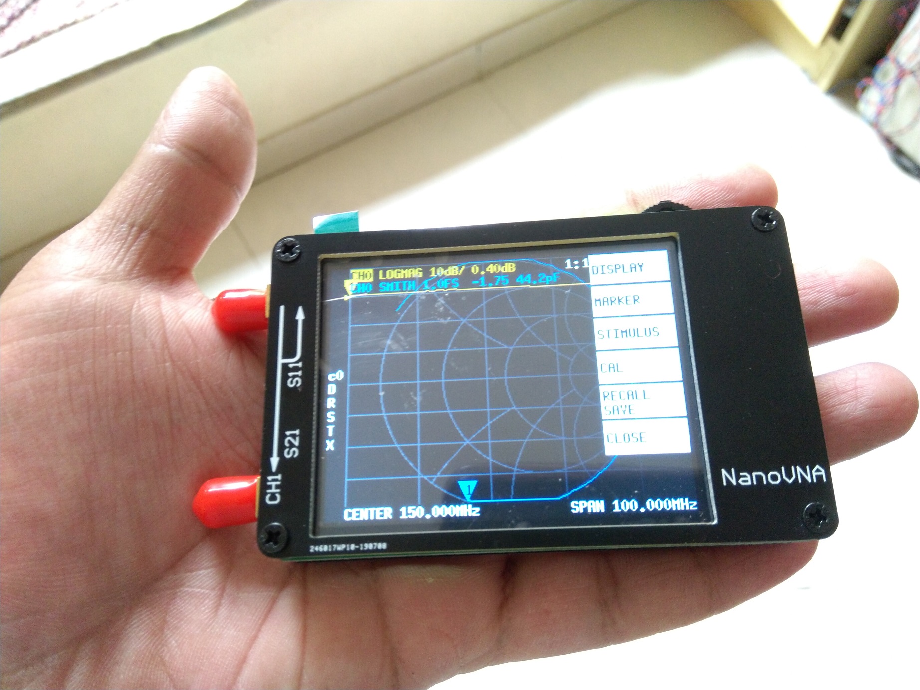
We have gone over NanoVNA so many times in the past. I did a complete review of the inexpensive NanoVNA last month. Furthermore, I compared it with the super-expensive Keysight N9952A Vector Network Analyzer. Finally, I wrote a small script to compute the TDR response from the S-parameter data that NanoVNA gave us. Today, I wrote a small extension to the TDR script to plot the impedance profile of a cable. In this article, we will go over the basic mathematics involved to compute the impedance profile and finally, you all get the script to try it out.
Understanding the concept
Computing TDR (time domain reflectometry) from frequency domain data results in what we call as the “impulse response”. In other words, it’s the response of the DUT (device under test) when we inject an impulse. In our previous test case where we used a segment of a cable as the DUT, the impulse went through the cable and reflected back from the open end. Remember that in our case, this impulse is imaginary because we are never sending it in the first place, instead synthesising it using the Inverse Fourier transform.
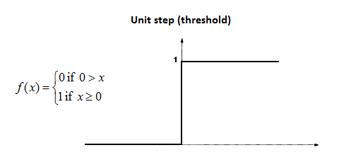
According to a Keysight Application note, we can derive the impedance profile of the cable if we obtain a step response instead of an impulse response. Now, what is a step response? The step response is when we apply a sudden step signal at the input of the DUT. A step looks like the sharp square wave except that the voltage transitions from 0V to 1V (or whatever volts) and stays there forever.
For those of you who don’t know, you can obtain a step response of the DUT if you already have the impulse response.
Finding impulse response and step response involve slightly advanced knowledge of signal processing. You can skip the following section.
In order to find the step response of any system, we need to convolve the impulse response with the step input.
\(y(n) = \sum_{k=-\infty}^\infty h(k)u(n-k)\)
Since, TDR response is \(0\) for \(n < 0\), the lower limit of the summation changes. Additionally, we are only interested in convolving up to \(N\) where \(N\) is the number of \(FFT\) points. Thus, the equation changes to the following
\(y(n) = \sum_{k=0}^\infty h(k)\)
Once we obtain the step response, we are very close to plotting the impedance profile. Remember, that the \(S_{11}\) is return loss. We need to convert return loss into impedance \(Z\).
To do so, we follow a simple derivation below.
\(S_{11} = \frac{ Z_{in} – Z_o }{Z_{in} + Z_o}\)
Therefore, rearranging the terms gives us an equation to compute \(Z_{in}\) from the \(S_{11}\).
\(Z_{in} = Z_o \biggr(\frac{1 + S_{11}}{1 – S_{11}}\biggl)\)
Now, let us try to implement this in Python.
Python implementation
As mentioned earlier, the TDR script gives us the impulse response of the DUT. We now compute the step response by adding a few lines in the script.
The steps:
- Create a step waveform (Basically all ones in an array)
- Convolve it with the impulse response
- Transform \(S_{11}\) to \(Z\)
- Truncate the step response to \(NFFT\) points
|
1 2 3 4 5 6 7 |
td = np.fft.ifft(s11, NFFT) # Create step waveform and compute step response step = np.ones(NFFT) step_response = np.convolve(td, step) step_response_Z = Zo * (1 + step_response) / (1 - step_response) step_response_Z = step_response_Z[:16384] |
The results
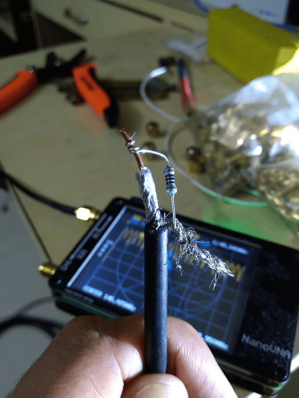
While testing this script, I created two test scenarios. One, with the short-circuited-ended cable. In another scenario, there are multiple cables with difference impedances and a \(50\Omega \) termination. The first cable is a \(50\Omega\) RG316, then a \(75\Omega\) RG6U and finally another \(50\Omega\) RG58. Finally, a \(50\Omega\) resistor terminates everything.
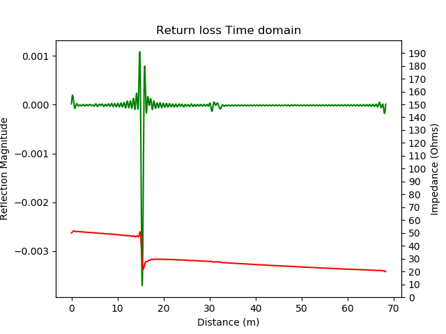
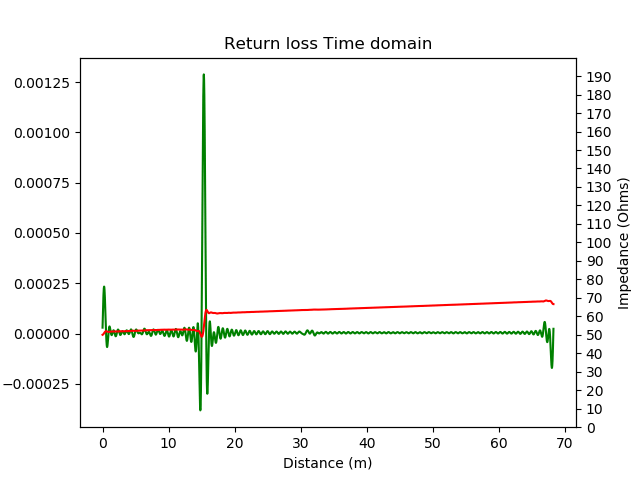
There are two things to observe above. The impulse response peak and the sudden spike in impedance align quite perfectly. The second thing to note here is that the open-ended cable shows a good \(50\Omega\) impedance until the point of short circuit. After the short circuit, the impedance settles down to \(0\Omega\).
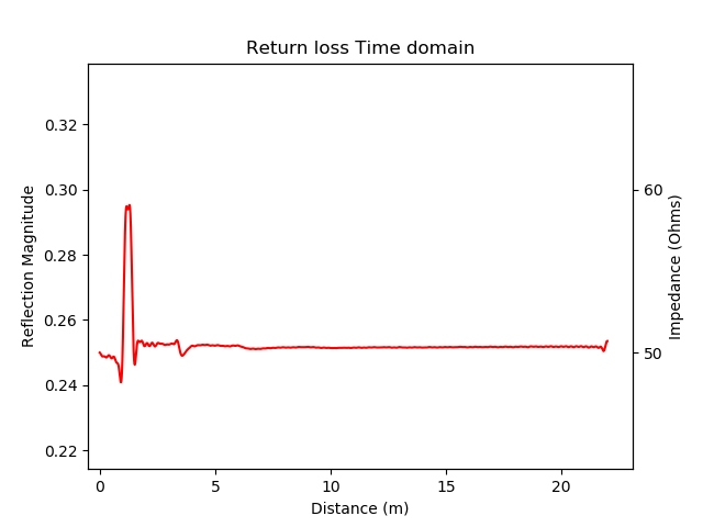
In the second image, we are looking at the second scenario, where there are cables having multiple impedances. To repeat, we have \(50\Omega,\thinspace 75\Omega \thinspace and \thinspace 50\Omega\) respectively. The graph starts at \(50\Omega\), jumps to \(60\Omega\) and finally returns back to slightly higher than \(50\Omega\). Eventually, it settles at \(50\Omega\) corresponding to the resistor value.
In another experiment, I terminated the cable end with \(100\Omega\) like shown below.
The full script is below.
|
1 2 3 4 5 6 7 8 9 10 11 12 13 14 15 16 17 18 19 20 21 22 23 24 25 26 27 28 29 30 31 32 33 34 35 36 37 38 39 40 41 42 43 44 45 |
import skrf as rf import matplotlib.pyplot as plt from scipy import constants import numpy as np raw_points = 101 NFFT = 16384 PROPAGATION_SPEED = 83 Zo = 50 _prop_speed = PROPAGATION_SPEED / 100 cable = rf.Network('step_response_experiment/cable_open.s1p') s11 = cable.s[:, 0, 0] window = np.blackman(raw_points) s11 = window * s11 td = np.fft.ifft(s11, NFFT) # Create step waveform and compute step response step = np.ones(NFFT) step_response = np.convolve(td, step) step_response_Z = Zo * (1 + step_response) / (1 - step_response) step_response_Z = step_response_Z[:16384] # Calculate maximum time axis t_axis = np.linspace(0, 1 / cable.frequency.step, NFFT) d_axis = constants.speed_of_light * _prop_speed * t_axis # find the peak and distance pk = np.max(td) idx_pk = np.where(td == pk)[0] print(d_axis[idx_pk[0]] / 2) # Plot time response fig, ax1 = plt.subplots() ax2 = ax1.twinx() ax2.set_ylim([0, 500]) ax2.yaxis.set_ticks(np.arange(0, 500, 50)) ax1.plot(d_axis, td, 'g-') ax2.plot(d_axis, step_response_Z, 'r-') ax1.set_xlabel("Distance (m)") ax1.set_ylabel("Reflection Magnitude") ax2.set_ylabel("Impedance (Ohms)") ax1.set_title("Return loss Time domain") plt.show() |
Let me know what you think about this script in the comments below.
If you haven’t purchased a NanoVNA yet, go ahead and get one. It’s worth it!
Very nicely done …good job Salil
Awesome post, thanks for sharing.
Saludos desde Ecuador…
Felicitaciones por excelentes aportes…
Puede guiarme o indicarme como corro los script
Very informative tidbit of code. Thank you for sharing.
if you change line 42 and 43 to:
ax1.set_ylabel(“Reflection Magnitude”).set_color(‘green’)
ax2.set_ylabel(“Impedance (Ohms)”).set_color(‘red’)
then the labels will match the plotted curve colors to make the connections a little more obvious
Hi Salil,
Thak you for sharing your works with us.
When i run the script with the open ended coax cable, the measurement and the plot coming correct, but when i run the script with the shorted cable’s s1p parameter, the plot shows the inverse peak at the right length,but the outcome of the script gives wrong measurement. Can you help me to deal with it?
I believe the inverse peak indicates 180 degree phase shift from the shorted point which is correct. I think the plot is showing “real+imag” instead of “abs(real, imag)”.
Thanks for the reply. I figure out that script includes a line to get max peak point at open ended cable. When shorted, the inverse peak occurs and script line should be corrected to get min peak point. And here is another question; Why did you take NFFT as 16384? What does that NFFT mean in our script? It’s 2^n, and n=14 but where did we get that 14 from?
Hi,
Note that scikit-rf also provides methods to make time domain calculations:
https://scikit-rf.readthedocs.io/en/latest/examples/networktheory/Time%20Domain.html